Freeze the Top Row or First Column
1. Click on the View tab on the Excel Ribbon.
2. Click the drop-down for Freeze Panes.
3. Click Freeze Top Row – allows scrolling down many rows and still shows the top row.
OR
4. Click Freeze First Column – allows scrolling to the right and still shows the first column.
Note: You cannot select both Freeze Top Row and Freeze First Column.
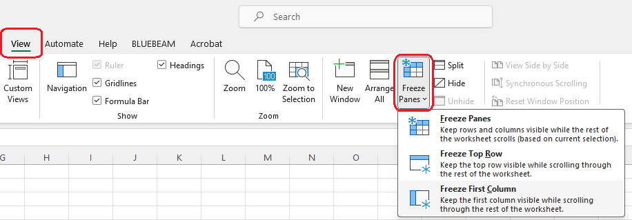
Freeze Panes
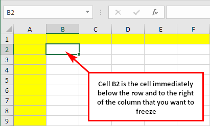
If you want to freeze both columns and rows, do the following:
1. If Split is currently active, turn it off.
2. If Freeze Panes is currently active, turn it off.
3. Select the cell below the rows you wish to keep visible and to the right of the columns you want to keep visible when you scroll.
4. Select Freeze Panes > Freeze Panes.
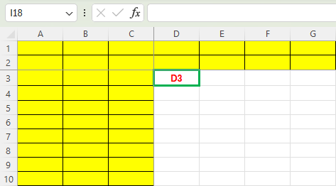
If you wish to freeze the top 2 rows and left 3 columns, D3 would be the cell immediately below row 2 and to the right of column C, you would select D3 before selecting Freeze Panes.
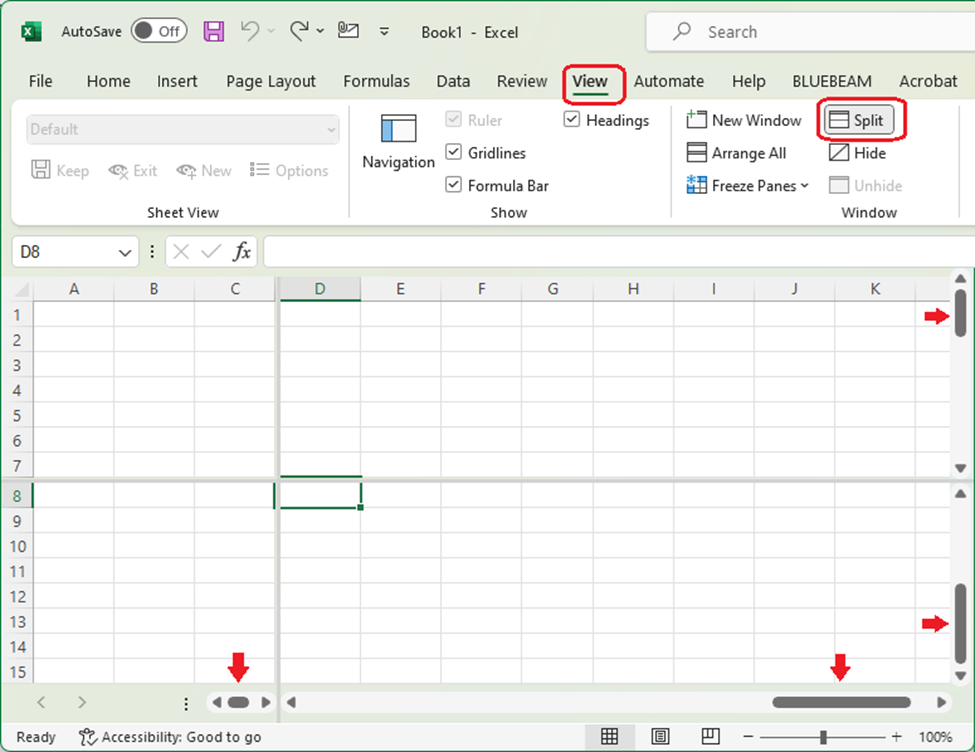
Split View
Split View places the spreadsheet in four different quadrants that are individually scrolled.
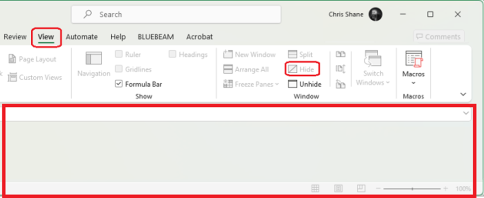
Hide & Unhide
Hides the workbook.
Unhide restores the workbook.
